Chapter 17: Nonlinear Support Vector Machines

Many classification problems warrant nonlinear decision boundaries. This chapter introduces nonlinear support vector machines as a crucial extension to the linear variant.

§17.01: Feature Generation for Nonlinear Separation

Linear functions are restrictive which can lead to underfitting. Alternatively we can use $\Phi_i$ to extend a linear classifier by projecting the underlying data into a higher dimensional feature rich space in which the data can be linearly separated. The goal of kernel methods is to introduce non-linear components to linear methods.
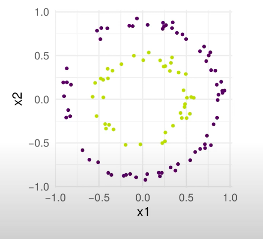
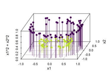
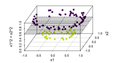
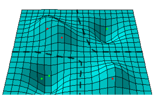
For example consider the following dataset where the two classes lie as concentric circle. There exists no linear classifier in the 2D case. However if we introduce a third dimension: $x_1^2 + x_2^2$, then you can see in the second figure how we now have “depth” and the dataset can be separated by a hyperplane.

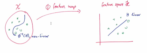
In essence what we are trying to do is find a feature map $\Phi$ such that a linear classifier exists in the newer feature space.
However for even small datasets, the extracted features can grow infeasibly and training SVM classifiers can prove to be computationally difficult and memory inefficient.

§17.02: The Kernel Trick

Recall the dual soft-margin SVM. In the transformed space the problem is:
\[\max_\alpha \Sigma_{i=1}^n \alpha_i - \frac{1}{2} \Sigma_{i=1}^{n} \Sigma_{j=1}^n \alpha_i \alpha_j y^{(i)}y^{(j)} <\Phi(x^{(i)}),\Phi(x^{(j)})> \\ \text{s.t.} \\ 0 \leq \alpha_i \leq C \\ \Sigma_{i=1}^n \alpha_i y^{(i)} = 0\]

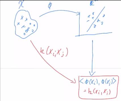
The key observation here is that our problem does not depend on the features itself but rather on the the pairwise inner-product of the inputs i.e. we don’t need to know the transformations directly but only need to know the product.
The entire idea behind the kernel method is to find a “shortcut” to directly calculate these inner products instead of first transforming and then calculating.

Thus, given some points in an abstract space $X$, the kernel function implicitly embeds the points into a higher dimensional space via a non-linear feature map $\Phi$. A (mercer) kernel on a space $X$ is a continuous function $k: X \times X \rightarrow \mathbb{R}$ with the following properties:
1. Symmetric: $k(x_i, x_j) = k(x_j, x_i)$
2. Positive Definiteness: $\forall x_1,…,x_n \in X$ and $c_i, c_j \in \mathbb{R}$ ,$\Sigma_{i=1}^n \Sigma_{j=1}^n c_i c_j k(x^{(i)}, x^{(j)}) \geq 0$ or rather The kernel Gram Matrix $K \in \R^{n \times n}$ with $K_{ij} = k(x^{(i)}, x^{(j)})$ is positive semi-definite.

Some properties of kernels:
1. For $\lambda \geq 0, \lambda .k$ is also a kernel
2. $k_1 + k_2$ is also a kernel
3. $k_1 \times k_2$ is also a kernel
For a test-point $x$:

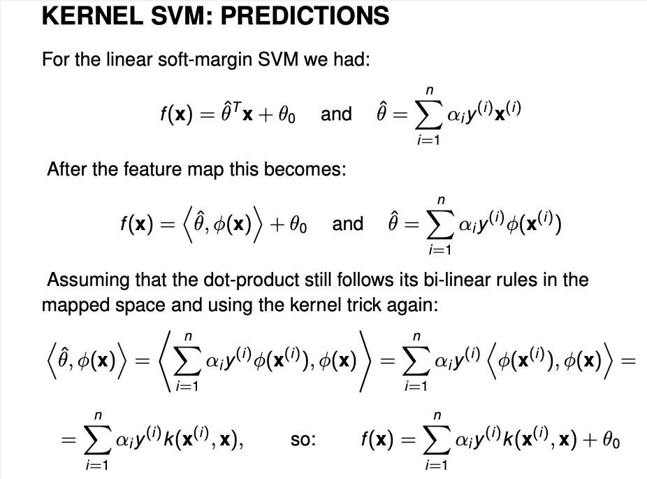
The kernel trick allows us to make linear machines non-linear in a very efficient manner. Linear separation in high-dimensional spaces is very flexible. Learning takes place in the feature space, while predictions are computed in the input space.

§17.03: The Polynomial Kernel

Homogenous Polynomial Kernel: $k(x,y) = (x^Ty)^d$. The feature map contains all monomials of exactly order d:
\[\phi(x) = (\sqrt{\binom{d}{k_1, ...,k_p}}x_1^{k_1},....,x_p^{k_p} )\]
Therefore for $p=d=2$:
\[\phi(x) = (x_1^2, x_2^2, \sqrt{2}x_1x_2)\]
Nonhomogenous Polynomial Kernel: $k(x,y) = (x^T y + b)^d$. The feature map contains all monomials upto order d:
\[\phi(x) = (\sqrt{\binom{d}{k_1, ...,k_{p+1}}}x_1^{k_1},....,x_p^{k_{p}}, b^{k_{p+1}/2} )\]
Therefor $p=d=2$:
\[\phi(x) = (x_1^2, x_2^2, \sqrt{2}x_1x_2, \sqrt{2b}x_1, \sqrt{2b}x_2, b)\]
The higher the degree, the more non-linearity in the decision boundary.

§17.04: Reproducing Kernel Hilbert Space and Representer Theorem

Mercer’s theorem says that for every kernel there exists an associated (well-behaved) feature space where the kernel acts as a dot-product
1. There exists a Hilbert space $\Phi$ of continuous functions $X \rightarrow R$ (think of it as a vector space with inner product where all operations are meaningful, including taking limits of sequences; this is non-trivial in the infinite-dimensional case).
2. and a continuous feature map $\phi : X \rightarrow \Phi$
3. Kernel computes the inner product of the features: $<\phi(x), \phi(\tilde{x})> = k(x,\tilde{x})$
There are many possible such Hilbert spaces and feature maps for the same kernel. However they are all isomorphic (”equivalent”). We take a look at reproducing kernel Hilbert space (RKHS).

§17.05: The Gaussian RBF Kernel

What makes the gaussian kernel so powerful is that we can approximate any arbitrary continuous function as a sum of Gaussians.
The “radial” Gaussian Kernel is defined as: $$ k(x, y) = \exp(-\frac{||x-y||^2}{2\sigma^2})$$

If we choose a large $\sigma$, then the width becomes large and we would need a very large number of such functions estimate the original function.
A large $\sigma$ (small $\gamma)$ leads to a very smooth decision boundary and in the limit is essentially a linear function.

With enough such narrow curves, we can more or less approximate all functions.
A small $\sigma$ (large $\gamma)$ would yield a very rough/wiggly decision boundary and in the limit will basically model each data point.

Thus the Gaussian Kernel is Universally consistent. The downside is, the underlying function class is huge since all continuous functions can be approximated and therefore it’s extremely important that they be regularised.
It also means that all finite datasets are linearly separable. Does it mean we should use hard-margins instead of soft-margin when using RBF kernel? No! Even in an infinite dimensional space, we don’t want to overfit the noise and allow for some margin-violators.
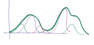
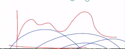
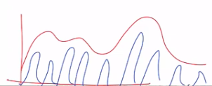
From the RKHS / Representer Theorem we know that decision for a test point $x$ is given by:
\[f(x) = \Sigma_{i=1}^n \alpha_i y^{(i)}k(x^{(i)}, x) = \theta_0\]

Only for the points which have $\alpha_i > 0$ i.e. the support vectors, RBF bumps are assigned. Since they are then multiplied by the labels (-1, +1), the bumps go up/down and this creates a rough decision surface And thus we can linearly separate the data.

§17.06: SVM Model Selection

“Kernelizing” a linear algorithm effectively turns this algorithm into a family of algorithms — one for each kernel. There are infinitely many kernels, and many efficiently computable kernels. SVMs are somewhat sensitive to its hyperparameters and should always be tuned.
Heuristic for RBF $\sigma$: Draw a random subset of data and compute pairwise distances between the points. Take a central quantile like the median. This relates the kernel width with the average distance between the points.