Chapter 5: Shapley

Shapley values originate from classical game theory and aim to fairly devide a payout between players. In this section a brief explanation of Shapley values in game theory is given, followed by an adaption to IML resulting in the method SHAP.

§5.01: Introduction to Shapley Values

Shapley values originate from cooperative game theory and provide a method to fairly distribute a total payout among collaborating players. In machine learning, this concept is adapted to explain individual model predictions by treating features as “players” that cooperate to produce a prediction.

Shapley Values in Game Theory

• In a cooperative game, for all possible players \(P = \{1,...,p\}\) each subset of players \(S \subseteq P\) forms a coalition. The payout of a subset/coalition \(S\) is mapped by the value function \(v: 2^{\mid P \mid} \rightarrow \mathbb{R}\).
  1. The payout of an empty coalition \(v(\emptyset) = 0\).
  2. The total achievable payout when all players cooperate is \(v(P)\).

• Some players might be contributing more than others in the coalition, and we need to determine a way to fairly distribute the payout i.e. find the marginal contribution of \(j^{th}\) player:

  \[\nabla(j, S) = v(S \cup j ) - v(S)\]
• In a cooperative game with no interactions i.e. the contribution of a player is the same regardless of the coalition, it is quite easy to figure out a fair distribution of the payout.
• However for a cooperative game with interactions, it is a bit unclear how to fairly distribute payouts since players contribute differently depending on the coalition.

• Averaging over the marginal contributions across different subsets may not always recover the total payout. This is because the value a player adds depends not only on who else is in the other coalition, but also on the joining order.

  Example of how joining order matters

  
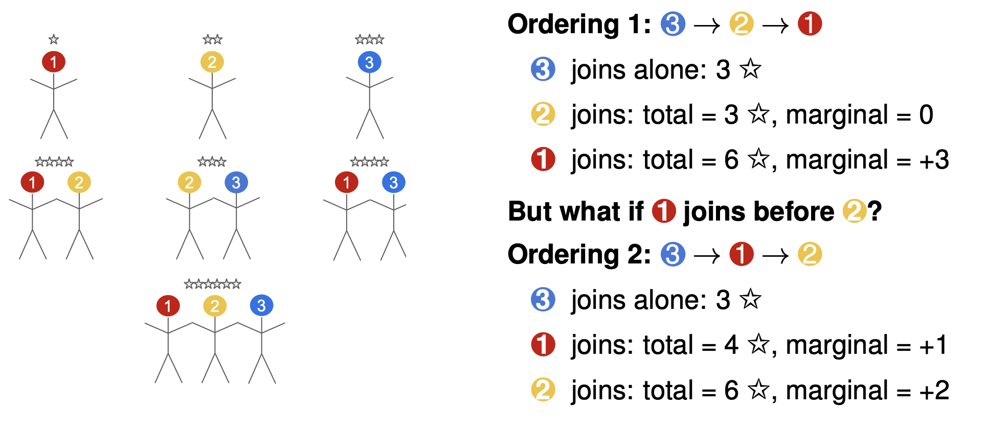
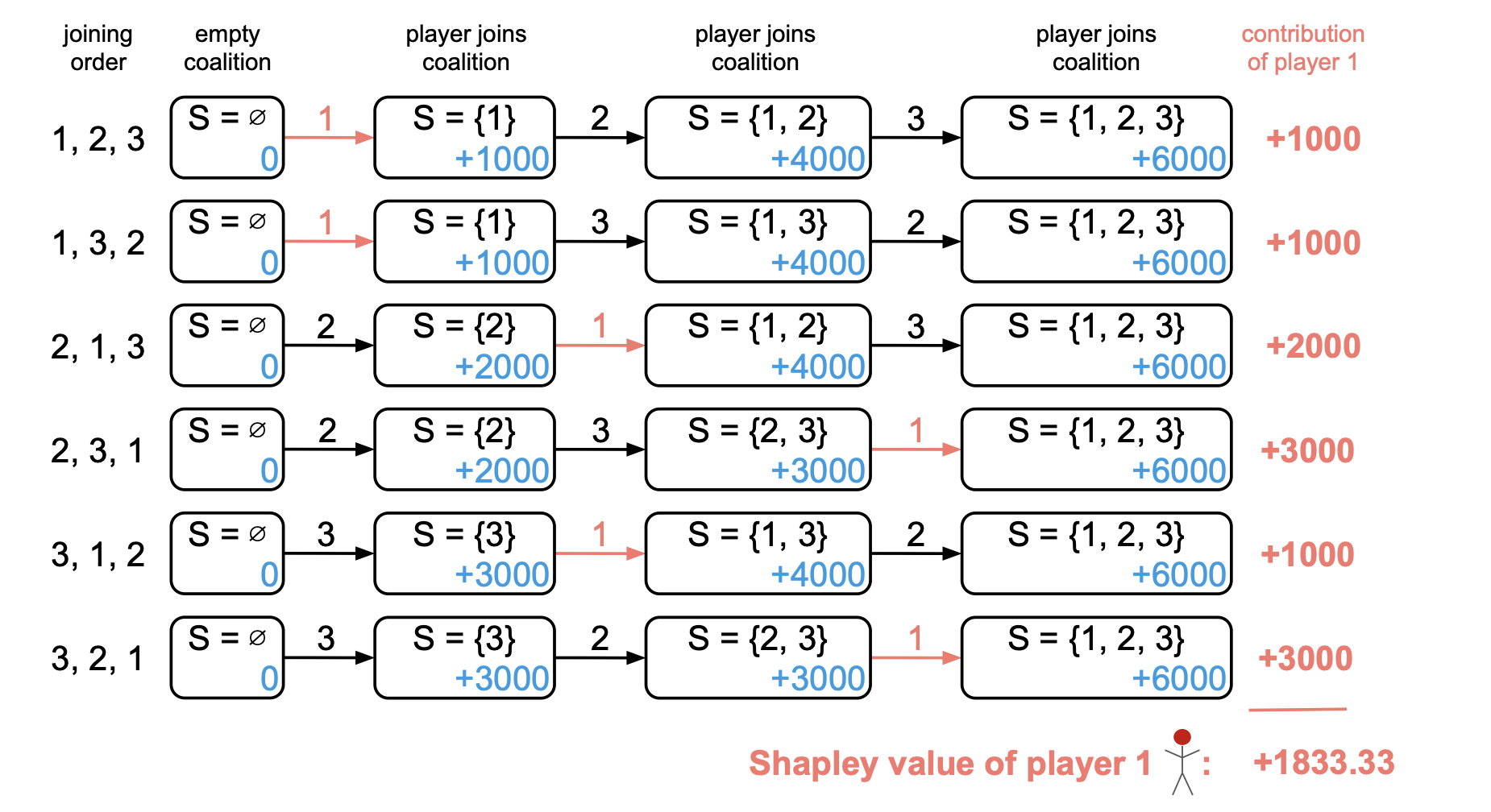
• The Shapley Value, averages each players contribution over all possible joining orders. It generates all possible joining orders of players (i.e. all permutations of \(P\)) and for each set, it tracks the player \(j^{th}\) marginal-contribution. Then the average of the \(j^{th}\) players marginal contribution over all joining orders is the Shapley value of the player:

• Formally the order definition of shapely value for player \(j\) is given by \(\phi_j\):

  \[\phi_j = \frac{1}{\mid P \mid !} \sum_{\tau \in \Pi} (v(S_j^\tau \cup \{j\}) - v(S_j^\tau))\]

  where \(\Pi\) is the set of all permutations and \(S_j^\tau\) is the set of players before \(j\) joins the ordering.

• This is usually computationally expensive as the number of orderings is \(\mid P \mid !\). Instead we can sample a fixed \(M \llless \mid P \mid !\) and average it out:

  \[\phi_j \approx \frac{1}{M} \sum_{\tau \in \Pi_M} (v(S_j^\tau \cup \{j\}) - v(S_j^\tau))\]

  where \(\Pi_M \subset \Pi\) is a random sampling of \(M\) player orderings.

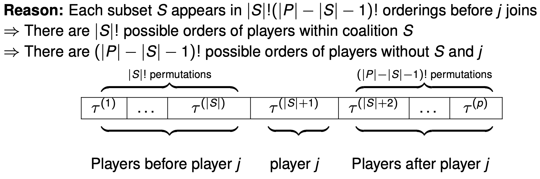
• Note however that the set \(S_j^\tau\) can occur in multiple permutations. If our player of interest was 3, then for the orderings \(\{1,2,3\}, \{2,1,3\}\), the set \(S_j^\tau = \{1,2\}\). The marginal contribution of the set \(\{1,2\}\) occurs twice because \(\{1,2,3 \}\) has two orderings in it whereby 3 joins last. More generally,

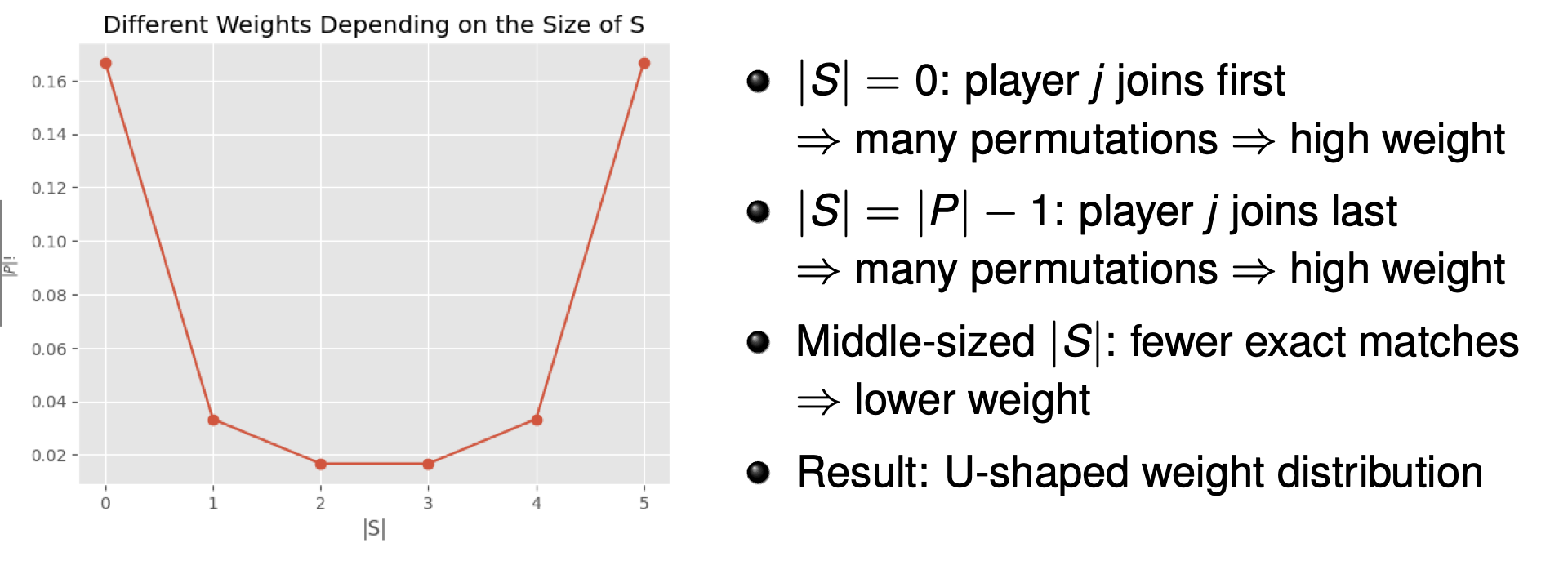
• The set definition is equivalent to the order definition, but is much quicker in computation. In the order definition, each term (order) had a weight of \(\frac{1}{\mid P \mid !}\). Instead now we look at each set which has a weight of \(\frac{\mid S \mid ! (\mid P \mid - \mid S \mid - 1)!}{\mid P \mid !}\).

  \[\phi_j = \sum_{S \subseteq P \ \{j\}}\frac{\mid S \mid ! (\mid P \mid - \mid S \mid - 1)!}{\mid P \mid !} (v(S \cup \{j\}) - v(S))\]

Axioms of Fair Payouts

The Shapley value provides a fair payout \(\phi_j\) for each player \(j \in P\) and uniquely satisfies the following axioms for any value function \(v\) :

1. Efficiency: The total payout \(v(P)\) is fully allocated to players:

   \[\sum_j \phi_j = v(P)\]
2. Symmetry: Indistinguishable players \(j,k\) receive equal shares i.e. \(\phi_j = \phi_k\).
3. Null Player: Players who contribute nothing, receive nothing.
4. Additivity: For two separate games, with value functions \(v_1, v_2\), define a combined game with \(v(S) = v_1(S) + v_2(S) \forall S \subseteq P\). Then:

\[\phi_{j, v_1 + v_2} = \phi_{j, v_1} + \phi_{j, v_2}\]

i.e. Payout of combined game = payout of the two separate games

---

§5.02: Shapley Values for Local Explanations

• Players? Game? Payout? What’s the connection to machine learning predictions and interpretability? Assume you’ve trained a machine learning model to predict apartment prices. For a certain apartment that has an area of \(50m^2\), is located on the \(2^{nd}\) floor, has a park nearby, and cats are banned, it predicts €300,000. If we need to explain this prediction, then we can use Shapely. But how?
  • The Game is simply the prediction task for a single observation of the dataset i.e. \(\hat{f}(x^{(i)})\).
  • The Players are the features which cooperate to produce a prediction i.e. \(x_j, j \in \{1,...,p\}\).
  • The Payout is the value of the prediction function with the selected features evaluated for the particular observation. Remember how the Shapely value of \(v(\emptyset) = 0\)? For that reason we consider the payout to be \(v(S) = \hat{f}_S(x^{(i)}_S) 0 - \hat{f}_\emptyset\). But how can we make a prediction using a subset of features without changing the model? \(\Rightarrow\) we use PD functions by marginalizing over \(x_{-S}\). Thus, we use \(\hat{f}_S = \int \hat{f}(x_S, x_{-S}) d P_{X_{-S}}\).
  • The Goal is to distribute the total payout \(v(P) = \hat{f}(x) - \hat{f}_\emptyset\) fairly among the features.

• The Shapely Value \(\phi_j\) quantifies the contribution of \(x_j\) via:

  \[\phi_j(x) = \frac{1}{\mid P \mid !} \sum_{\tau in \Pi} f_{S_j^\tau \cup \{j\}}(x_{_{S_j^\tau \cup \{j\}}}) - f_{S_j^\tau}(x_j^\tau)\]

  i.e. \(\phi_j\) quantifies how much feature \(x_j\) contributes to the difference between the prediction \(\hat{f}\) and mean-prediction \(\hat{f}_\emptyset\)

• Since the exact computation \(\hat{f}_S(x_S) = \frac{1}{n} \sum_{1}^n \hat{f}(x_S, x_{-S}^{(i)})\), calculating the exact shapely value is impractical and infeasible when the number of features increase since the number of orders grows factorially. For example, 10 features yields 3.6 million orderings. Furthermore, within each ordering we need to compute a PD-function which is an n-valued sum, therefore the total computations required is \(\mid P \mid ! \dot n\)
• Instead we can use \(M\) random samples of permutation \(\tau\) and data points. Larger the \(M\), better our approximation ofcourse. We can implement the algorithm as follows:

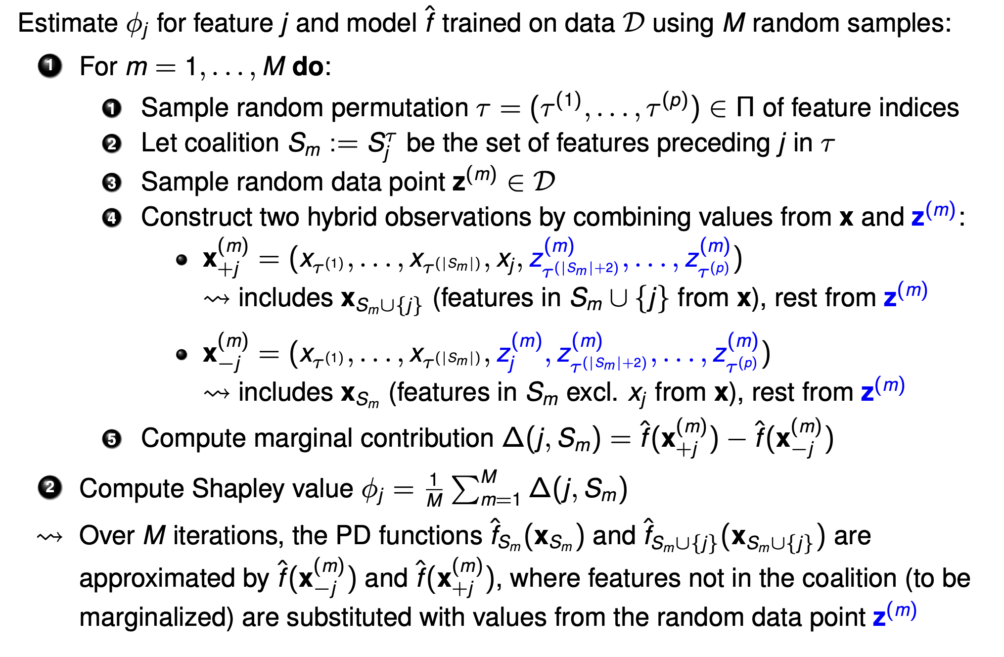
An important thing to note here: For the calculation of marginal contribution, the value of all preceding features + value of feature j is taken from \(x^{(i)}\) and the remaining from a random point and it is compared against taking all feature values preceding j being taken from \(x^{(i)}\) and the rest including \(j^{th}\) feature value being taken from a random point.

Axioms for Fair Attribution

1. Efficiency: Sum of Shapley values add up to the centered prediction: \(\sum_{1}^p \phi_j(x) = \hat{f}(x) - \mathbb{E}_x[\hat{f}(x)]\) i.e. all predictive contribution is fully distributed and accounted for among the features.
2. Symmetry: Identical contributors receive equal value.
3. Null Player: Irrelevant features receive 0 value i.e. if \(\hat{f}_{S \cup \{j\}}(x_{S \cup \{j\}}) = \hat{f}_S(x_S) \Rightarrow \phi_j = 0\).
4. Additivity: Attributions are additive across models which enables combining shapley values model ensembles.

All in all, Shapley Values have a strong theoretical foundation from cooperative game theory, produce fair attribution, and also provide contrastive explanations by quantifying each features role in deviating from the average prediction. However they come at a huge computational cost and are not robust to correlated data.

---

§5.03: SHAP: Shapley Additive Explanation Values

• SHAP expresses the prediction of \(x\) as a sum of contributions from each feature:

  \[g(z') = \phi_0 + \sum_{j=1}^p \phi_j z^{'}_j\]

  where \(z' \in \{0,1\}^p\) i.e. it is a \(p-\)dimensional vector with \(z^{'}_j = 1\) if feature \(j\) is present in the coalition, 0 otherwise (influence of \(x_j\) is to be marginalized out).

• We fit a surrogate model \(g(z')\) satisfying Shapley axioms and recovering \(\hat{f}(x)\) when all features are present (i.e. \(\mathbf{z'} = \mathbf{1}\)). Evaluation of \(g(z')\) can be done in one of two ways:

  1. \(g(z') \approx E[\hat{f}(X) \mid X_s = x_s]\) :
     • This is the conditional expectation of the model output \(f(X)\) given that the features in \(S\) are fixed to their values in the observation of interest (\(x_S\)) i.e. the average prediction you would get if you considered all possible values for the features not in \(S\) weighted by their conditional probability.
     • This approach respects statistical dependencies between the features (i.e. for correlated features only realistic combinations would be considered).
     • If we fix these features to their values in our observation, and let all the other features vary according to how they are distributed in the data (but always in a way that’s consistent with the fixed features), what is the average model prediction?
  2. \(g(z') \approx E_{X_{-S}}[f(x_S, x_{-S})]\) :
     • This is the average prediction you would get if you paired the fixed values \(x_S\) with all possible values of the other features, assuming the features in \(S\) and not in \(S\) are independent breaking correlation between the features leading to unrealistic evaluation points.
     • Here, you still fix the values of the features in \(S\) as before, but now, you let all the other features vary independently according to their overall (marginal) distribution in the data, ignoring any dependencies with the fixed features.

SHAP Framework

• SHAP is accurate locally i.e. if the coalition includes all inputs then it is equivalent to the models original output (axiom of efficiency).
• Missingness: A missing feature gets an attribution of 0
• Consistency: If a model changes such that the marginal contribution of a feature value increases, then the corresponding Shapely value also increases
• Additivity, Dummy, and Symmetry follow.

Kernel SHAP

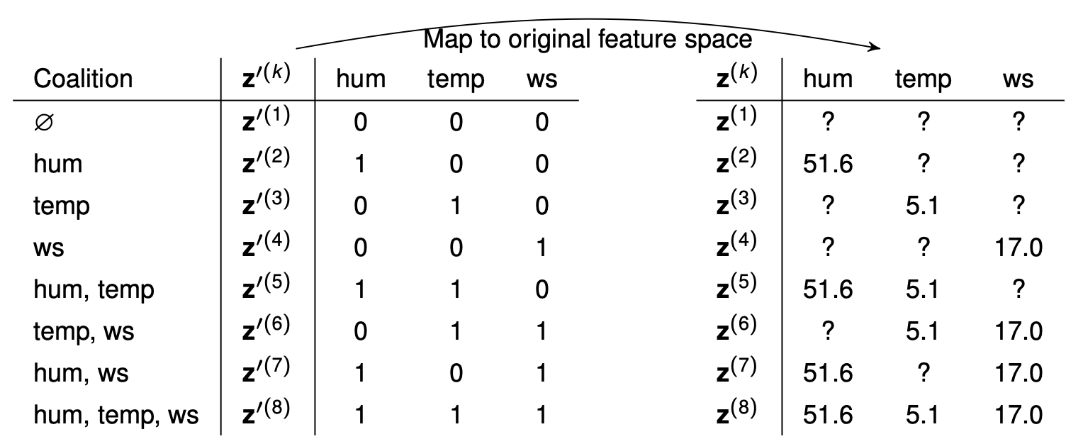
Suppose our point of interest is \(\mathbf{x} = (51.6, 5.1, 17.0)\)

Step 1: From all possible coalitions (\(2^p\)), we sample \(K\) from the simplified binary feature space. \(z^{'(k)} \in \{0,1\}^p\) indicates which features are present in the \(k^{th}\) coalition. This then needs to be mapped to the original space:

Step 2: For a each coalition vector (say \(\mathbf{z'} = (1,0,0)\)), the features that are not part of the coalition need to be marginalized out. We draw multiple background samples, keep the original feature value for \(x_0\), and the rest are taken from the background data. This is done \(B\) times: \(E_{X_{-S}}[f(x_S, X_{-S})] \approx \frac{1}{B} \sum_{b=1}^B \hat{f}(h_{x,x^{'(b)}}(z'))\) where \(h_{x,x^{'(b)}}(z')\) keeps the original feature values for those in the coalition and takes a background sample for the rest.

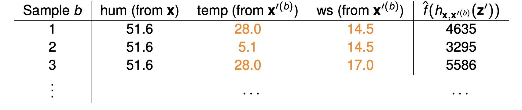
• If we use conditional distribution for the background sample, we get Observational SHAP, and if we use the marginal then we get Interventional SHAP.

Step 3: Compute the kernel weights for the surrogate model since we learn the most about a feature’s effect when it either appears in isolation or in near-complete context.

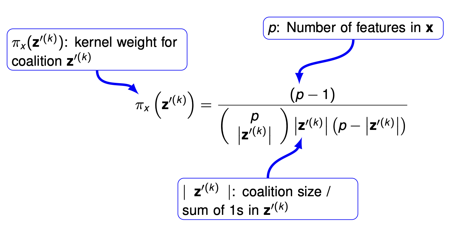
• Empty and full coalitions receive \(\infty\) weight.

Step 4: Fit a weighted linear model:

\[g(z') = \phi_0 + \sum_{j=1}^p \phi_j z_j^{'}\]

The weighted least-squares objective is then given by:

\[\min_\phi \sum_{k=1}^K \pi_x(z^{\(k)})[\hat{f}(h_x(z^{'(k)})) - g(z^{'(k)})]^2\]

where

\(\phi_0 = E[\hat{f(x)}]\) and \(\sum_{j=1}^p = \hat{f}(x) - \phi_0\)

The coalitions with \(\infty\) weights (i.e. \(\mathbf{z'}=1\) or \(\mathbf{z'} = 0\)) are instead used as constraints ensuring local accuracy and missingness.

Step 5: Return SHAP values: Estimated Kernel SHAP are equivalent to Shapley values. An important thing to note is that the weights of the Kernel SHAP are NOT the same as the weights from the Shapely Set definition.

Global SHAP

• We can run SHAP for every observation and get a \(n \times p\) matrix of Shapley values. Averaging the absolute value of the Shapley values for each feature over all observation (i.e. column-wise averages) gives us a “Feature Importance” metric:

  \[I_j = \frac{1}{n} \sum_{i=1}^n \mid \phi_j^{(i)} \mid\]
• Shapley FI does not provide information about the direction, only magnitude.

• An important thing to note here is that Shapley FI is based only on model predicitions where as others are often based on model’s performance/loss. This means if you have a poor model, the the Shapely FI gives us the FI based on this model. The ones based on performance use the ground truth.

• We can also plot the SHAP Dependence plot which shows the marginal effect similar to PD plot.